Plot Example: AT68 (Reliability-Based Failure Assessment Diagram)

This page shows how to plot a reliability-based failure assessment diagram (RFAD) and how to read it. An RFAD shows how the reliability changes when the parameters of two stochastic variables change, for example the mean load and the mean resistance. Brinkpy has no separate plotting command, so the plots come from an analyze run with the --plot-rfad (-r) flag. This page covers only the plots. For the reliability results of an analyze run, see FORM Only.

How to Generate the Plots

Add an RFADplot block to the problem file (see RFADplot), then add --plot-rfad (-r) to an analyze command:

brinkpy analyze -r

The RFAD is available only with analyze. Brinkpy builds a grid over the two parameters and runs a FORM analysis at every grid point. It then plots the probability of failure, the reliability index, and the alpha value of each stochastic variable over the grid.

Run Context

Problem module:

• problems/AT68Problem.py

Recorded result set:

• results/2026-11-03/19-00-27/AT68-ecb10.xlsx
• results/2026-11-03/19-00-27/AT68-ecb10.json
• results/2026-11-03/19-00-27/AT68-ecb10.py
• results/2026-11-03/19-00-27/AT68-ecb10.pickle
• results/2026-11-03/19-00-27/AT68-ecb10.pdf
• results/2026-11-03/19-00-27/profile-ecb10.yaml

Profile and run mode from saved profile:

• Profile used: default
• run_type: analyze
• plot_rfad: true

For results-folder and filename conventions, see CLI Result Files.

Equivalent command:

brinkpy analyze -r

Problem File Used

Source: Ang, A. H-S. and Tang, W. H., Probability Concepts in Engineering Planning and Design, Vol. II, Wiley, 1990, p. 363, Problem 6.8.

AT68Problem.py defines three uncorrelated stochastic variables, Y and Z (lognormal) and M (Gumbel maximum). The limit state function is g = Y * Z - M, with resistance R = Y * Z and load L = M. See Probability Density Functions for the full definition.

The RFADplot block sweeps the mean of Y on the x axis and the mean of M on the y axis:

"RFADplot": {
    "x_var": "Y",
    "x_param": "mean",
    "x_lim": [10.0, 70.0],
    "x_func": lambda S, D: S[0] * S[1],
    "x_label": "Resistance: \\mu(Y)*\\mu(Z)",
    "y_var": "M",
    "y_param": "mean",
    "y_lim": [500.0, 1500.0],
    "y_func": lambda S, D: S[2],
    "y_label": "Load: \\mu(M)",
},

Brinkpy varies the mean of Y from 10 to 70 and the mean of M from 500 to 1500. Every other parameter keeps its value from StochasticVariables. x_func and y_func receive the means and change only what the axes show: the x axis shows the mean resistance μ(Y) * μ(Z), from 500 to 3500, instead of μ(Y).

The standard deviation stays fixed

When Brinkpy changes the mean of a variable, it keeps the standard deviation, not the coefficient of variation. In this example the standard deviation of Y stays 5 and that of M stays 200 over the whole grid. At μ(Y) = 10, the coefficient of variation of Y is 0.5, while at μ(Y) = 70 it is about 0.07.

Changing one parameter at a time shows its effect on the reliability by itself. To study another parameter, set x_param or y_param to "std" (the standard deviation), "param1", or "param2" (the distribution parameters listed in Supported Statistical Distributions).

With the default profile, the grid has 30 × 29 = 870 points, so this run made 870 FORM analyses. The run took about 5.4 seconds.

How to Read the Plots

• Surface: the plotted quantity over the grid, colored by its value. The lines on the surface are contour lines of constant value.
• BP (base point): the means defined in StochasticVariables, here μ(Y) * μ(Z) = 2000 and μ(M) = 1000. Its value matches the FORM result of a normal analyze run.
• Views: with view: auto, Brinkpy chooses the viewing angle for each figure, so the axes may point in different directions from one figure to the next. Check the axis labels before comparing figures.

Generated Figures

The PDF result file for this run is saved as results/2026-11-03/19-00-27/AT68-ecb10.pdf. Because analyze always runs FORM, the file starts with the importance factors plot as Figure 1 (see FORM Only). The RFAD plots follow as Figures 2 to 6.

Figure 2: Probability of Failure

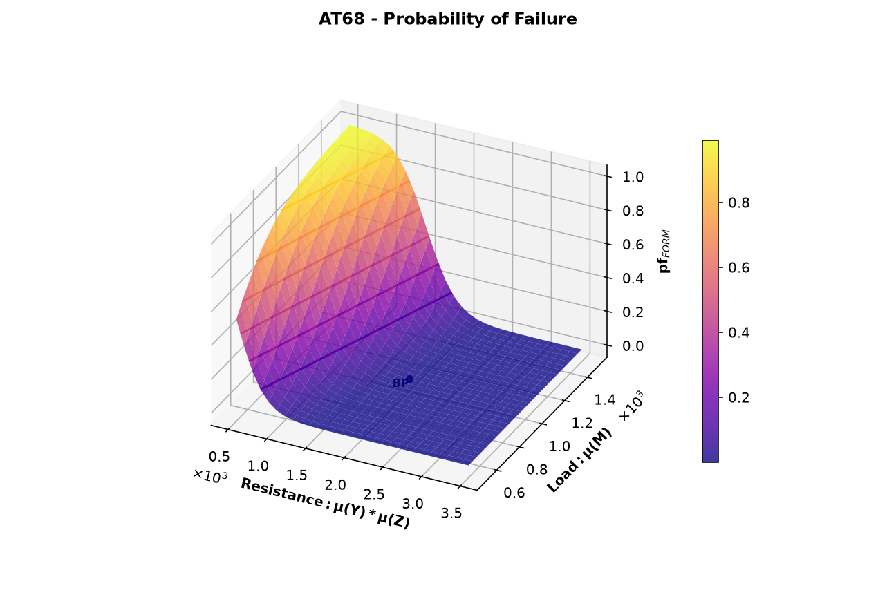
The FORM probability of failure over the grid. It is close to zero for most of the grid and rises steeply toward 1 where the mean resistance is small and the mean load is large. At the base point, pf = 0.0031. Because most of the surface is nearly flat at zero, the reliability index in Figure 3 is easier to read.

Figure 3: Reliability Index

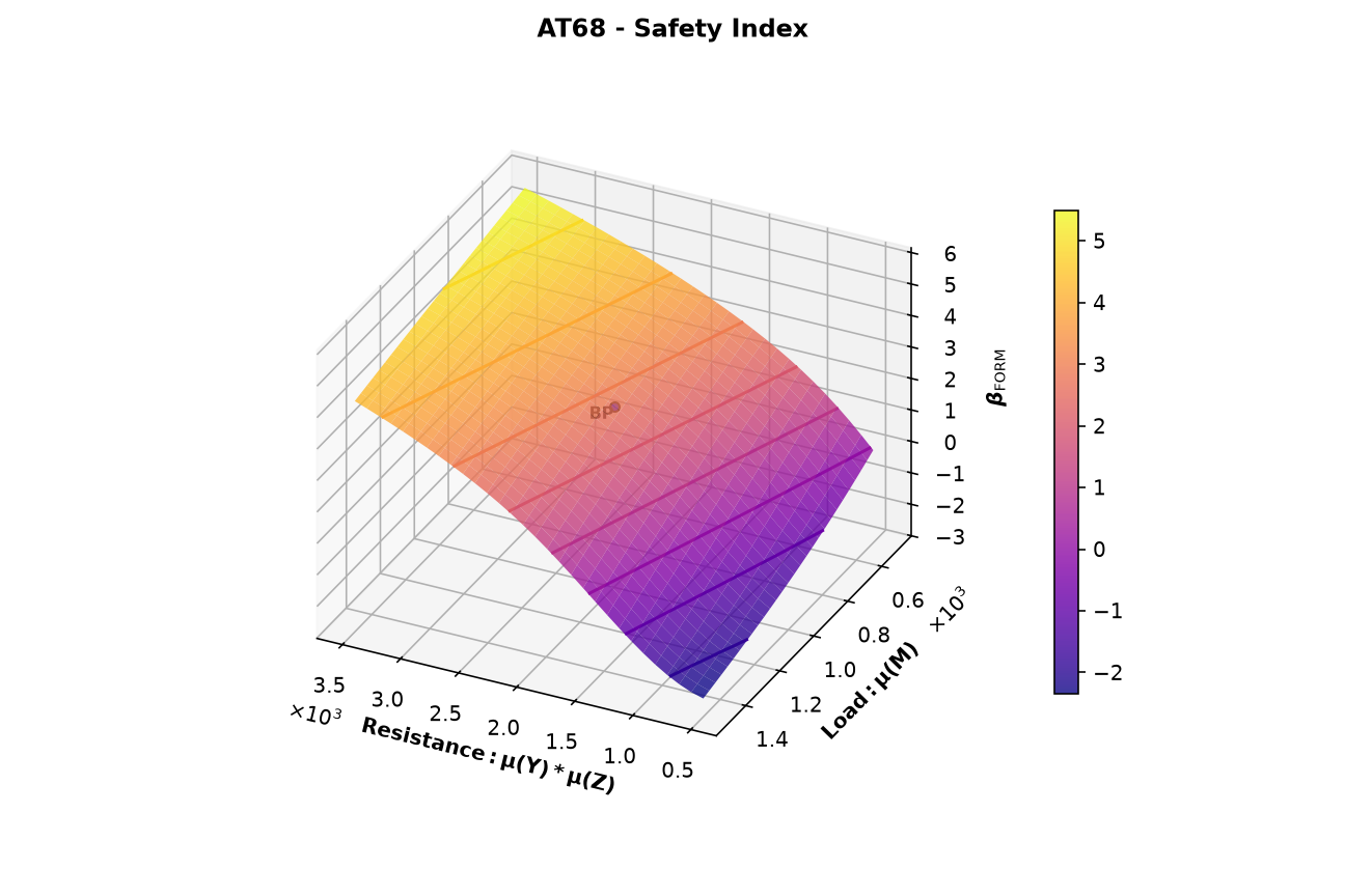
The FORM reliability index over the grid, from −2.4 to 5.6. Brinkpy titles this figure "Safety Index". At the base point, β = 2.742. A negative β means that the mean point is already in the failure region, so the probability of failure is larger than 0.5.

The contour lines are lines of constant β, drawn at whole numbers. They answer design questions directly. For example, along μ(M) = 1000 the β = 3 contour crosses at a mean resistance of about 2130, that is, μ(Y) ≈ 42.7. To reach β = 3 with a mean load of 1000, the mean of Y must be about 42.7 instead of 40.

Figures 4 to 6: Alpha Values

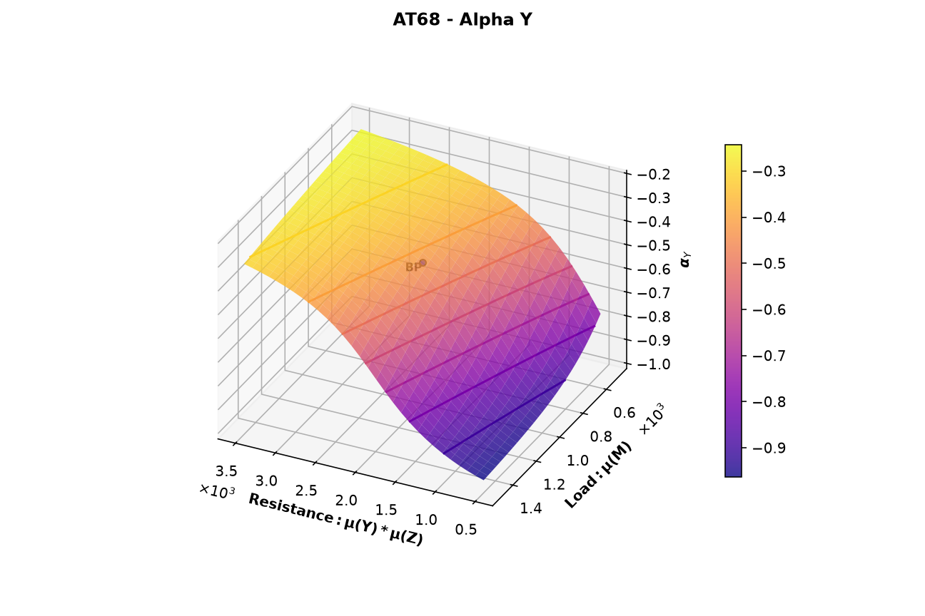
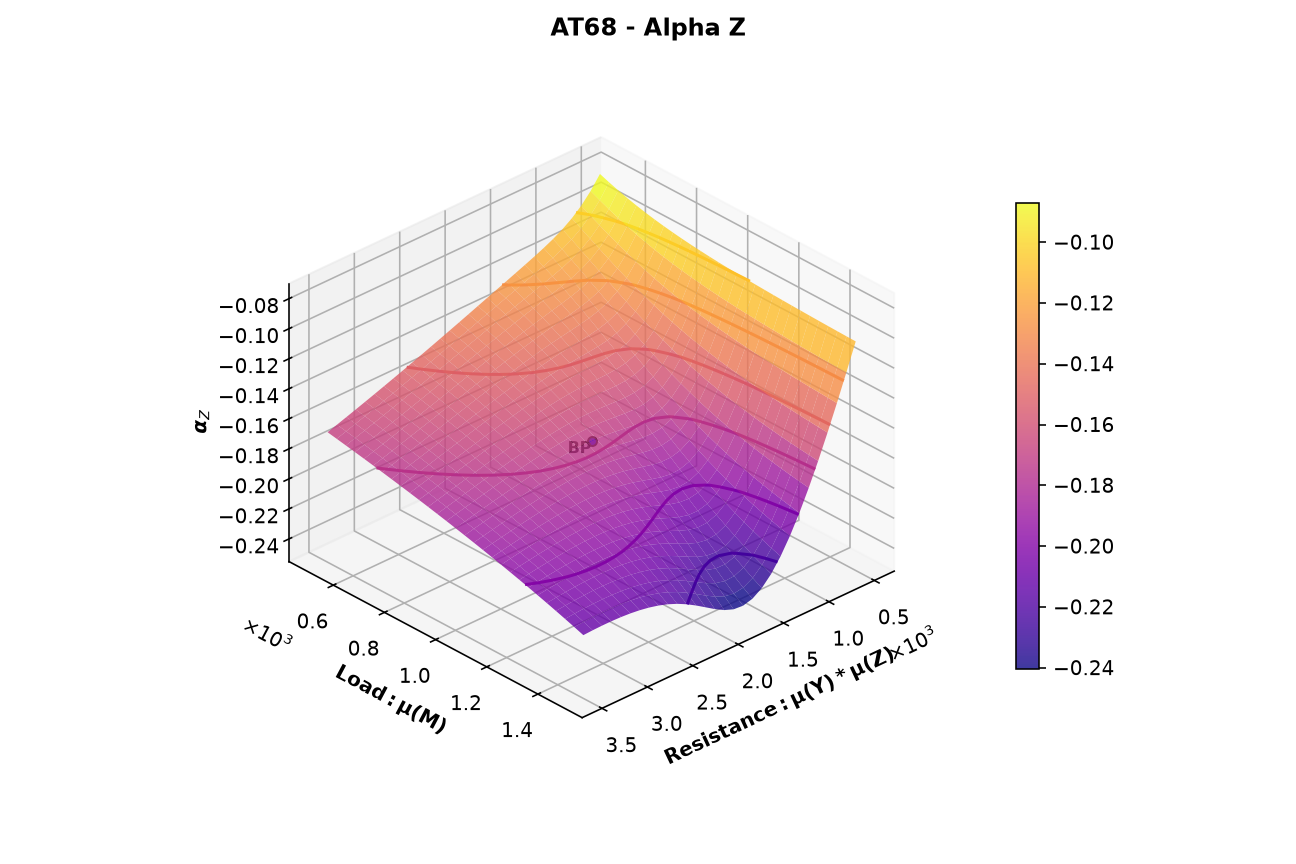
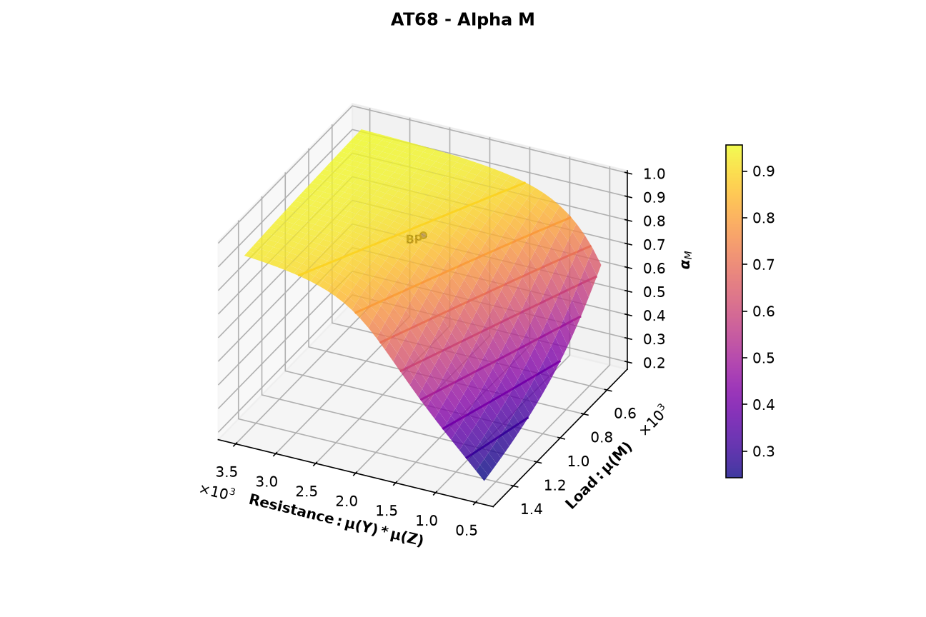
One figure per stochastic variable shows its alpha value, the component of the unit vector from the origin to the failure point in standard normal space. With the default alpha_direction: outward, the resistance variables Y and Z have negative alpha values and the load M has positive values. At the base point, α(Y) = −0.43, α(Z) = −0.17, and α(M) = 0.89, the same values as in the importance factors plot. At every grid point, the squares of the alpha values add up to 1.

The alpha values show which variable controls the reliability in each part of the grid:

• Where the mean resistance is large and the mean load is small, α(M) is close to 1. The load controls the reliability.
• Where the mean resistance is small, α(Y) approaches −1 and α(M) drops to about 0.2. With its standard deviation fixed at 5, Y becomes relatively more uncertain as its mean drops, so it takes over.
• α(Z) stays small, between −0.24 and −0.08, over the whole grid. Z has the smallest coefficient of variation (0.05) and never controls the reliability.

Profile Options

The rfad_plot_options section of the profile controls how the plots are drawn. This run uses the defaults:

rfad_plot_options:
  n_x_points: 30
  n_y_points: 29
  plot_beta: true
  plot_alphas: true
  plot_base_point: true
  with_labels: true
  ignore_axis_funcs: false
  view: auto
  cmap: plasma
  type: surface

Option	What to change it for
n_x_points, n_y_points	A finer or coarser grid. Brinkpy runs one FORM analysis per grid point (n_x_points × n_y_points), so the run time grows with the number of points.
plot_beta	Skip the reliability index plot (Figure 3) with false.
plot_alphas	Skip the alpha plots (Figures 4 to 6) with false.
plot_base_point	Hide the base point with false.
with_labels	Hide the BP label with false.
ignore_axis_funcs	Plot the swept parameters directly with true, ignoring x_func and y_func. In this example the x axis would show μ(Y) instead of μ(Y) * μ(Z).
view	The viewing angle of the 3D plots. auto (the default) chooses the elevation and azimuth that best show the details of each figure. default uses the Matplotlib default view. XY, XZ, and YZ look straight at that plane, and the versions with a minus sign (for example -XY) look at it from the opposite side. A tuple sets the elevation, azimuth, and roll in degrees, for example (30, 120, 0). With XY, the plots look like a classic contour map of the two parameters.
cmap	The colormap of the surfaces, as a Matplotlib colormap name.
type	contour to draw only the contour lines, still in a 3D plot, instead of the shaded surface.

To change these options, create a custom profile and run it by name, for example brinkpy analyze myprofile -r. See Profiles and RFAD Plot Options for the allowed values.